Dr Peter Woitke
The following pages contain lecturing material selected for advanced higher students at secondary schools in Scotland. The material was collected for and presented at the INSET-meeting at Kirkcaldy High School, November 13, 2015. Credits to Dr Aleks Scholz (lecturer AS1001), Dr Anne-Marie Weijmans (lecturer AS1101) and Prof Moira Jardine for providing material from their university courses.Download here as .odp (OpenOffice powerpoint) or here as .pdf
(the files contain movies which appear as big grey boxes marked by “?” and will not work, unfortunately)
(however, you can click on links provided below to download those movies)The presentation contains some questions marked in blue which you might want to ask and answer yourself, or to discuss with your students. You can find my answers here.
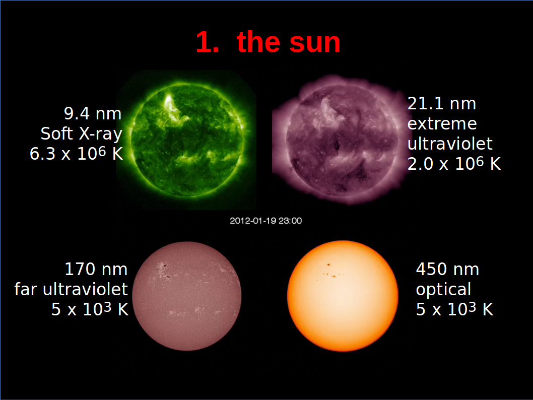 We start our journey from stars to the cosmic cycle of matter with the star we know the best – our sun. The optical image (lower right) shows the appearance of the sun’s photosphere, from which the majority of radiative energy is released into space, with the typical limb-darkening and a few sun spots. At shorter wavelengths (far UV, extreme UV, soft X-ray), we mostly see the outermost hot layers surrounding the sun, the chromosphere and the corona, where temperatures are as high as a few millions of Kelvin. At the shortest wavelengths, the photosphere is too cold to produce any significant emission.
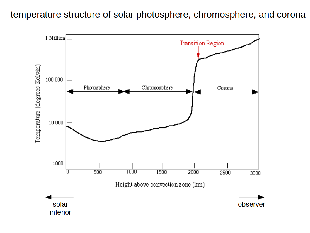
Sketch of the mean temperature as function of height above the convective layer which forms the footpoint of the solar photosphere. Note that the photosphere is characterised by a negative temperature gradient, before there is an inversion in the chromosphere, followed by a quite sudden transition into the much hotter and thinner corona.
Image Credit: Adapted by M.B. Larson from Sun, Earth, Sky by Kenneth Lang.
the dynamic sun
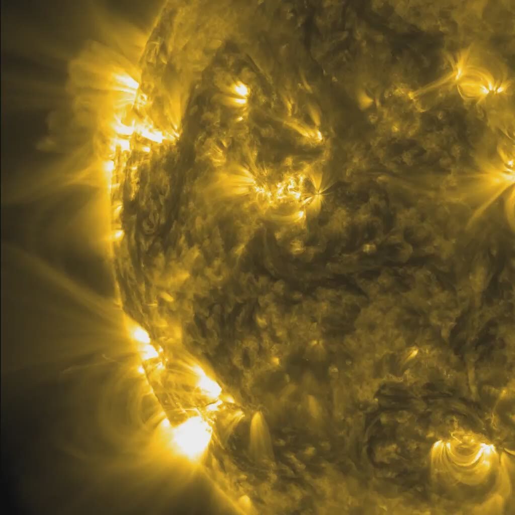
The picture shows that magnetic field lines emerge preferentially from sun spots, forming “coronal loops” in the corona where hot and highly ionised gas is trapped in the magnetic field, emitting hard UV photons and X-rays. The movie furthermore shows the rotation of the sun, and shows that the corona is far from being a stationary phenomenon. Compare the radial extension of this figure (the solar radius is Rsun ~ 700 000 km.) with the radial extension of the temperature structure shown in the above figure (~ 3000 km), showing that the photosphere of the sun is indeed extremely thin.
Credits: Solar Dynamics Observatory, NASA, download movie here.
solar flares and coronal mass ejections

Spectacular mass ejection events observed by the Solar Dynamics Observatory. Coronal Mass Ejections (CMEs) typically last a few hours and produce solar storms with velocities of up to a couple of 1000 km/s. The physical mechanisms leading to these events are not exactly known, but seem related to instabilities in the magnetic field, causing sudden re-connections of the twisted field lines. The sudden changes of the magnetic field induce strong electric fields, along which the ionised plasma is accelerated.
Video from the Solar Dynamics Observatory, NASA, see YouTube channel “SpaceRip”, download the movie here.
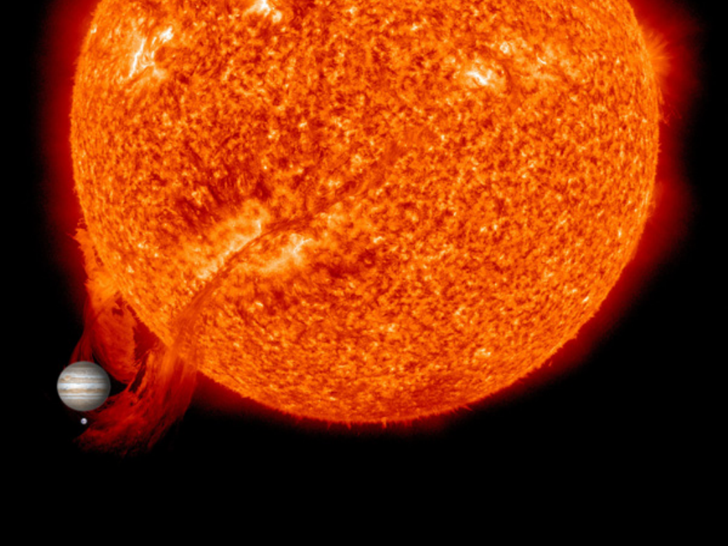 A solar prominence with Jupiter and Earth to size. Image Credits: Wikipedia.
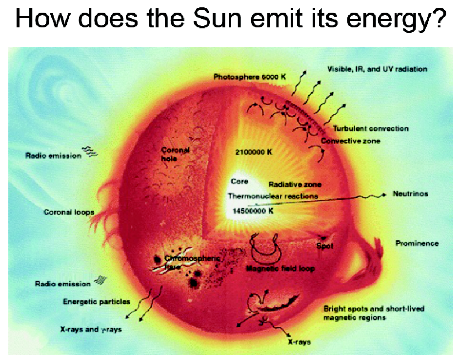 Image Credits: NASA.
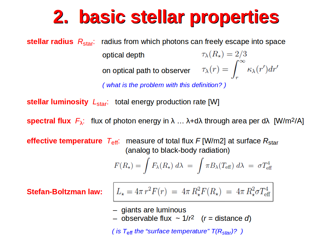 The opacity κλ = 1/lλ [1/m] describes the opaqueness of a medium; lλ is the mean free path of photons of wavelength λ in that medium. The integral over the opacity along a photon path is called the optical depth τλ. Photons emitted from radius r have probability exp(-τλ(r)) to escape the star when emitted radially. Taking into account that photons can also exit the star at slanted angles (not necessarily radially), the layer at τλ = 2/3 is found to contribute most to the emerging flux (Eddington-Barbier approximation). Therefore, τλ(Rstar) = 2/3 is the proper definition of the stellar radius.
The effective temperature of the star Teff is defined via the total radiative flux that emerges from the stellar atmosphere per unit area. Considering an analog black body sphere of radius Rstar, whose total radiative flux is given by the Stefan-Boltzmann law as F=σT4, we define Teff as the temperature of an analog black body which would produce the same total flux.
Using the definition of the luminosity as integral of the total flux over the stellar surface results in the Stefan-Boltzmann law in the form Lstar = 4π Rstar2 σTeff4.
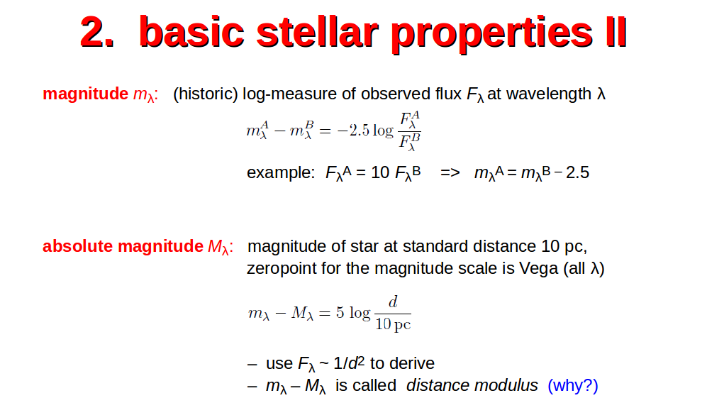 The brightness of stars are measured in magnitudes, and depends on wavelength. Concerning the wavelengths, broad standard photometric filters are applied, for example “ultra-violet” U (λ~365 nm), “blue” B (λ~445 nm), “visual” V (λ~550 nm), “red” R (λ~660 nm), “infra-red” I (λ~805 nm). The unit magnitude is derived from a system first used by the Greek astronomer Hipparcos (2nd century BC). In his catalogue of stars, 1st magnitude are the brightest stars, 6th magnitude are the stars just visible for the human eye. The relation to the physical flux Fλ was established later by realising that the human eye has a logarithmic sensitivity, and the factor 2.5 was adjusted to get similar results as Hipparcos.
In practise, magnitudes are not measured in an absolute way, but relative to standard stars, that’s why there are two objects A and B in the above equation. A could be the standard star (with known mλ), and B could be the star which magnitude we want to measure.
The absolute magnitude Mλ is obtained by moving the star to a standard distance of 10 pc, use Fλ ~ 1/d2 to derive the second from the first equation. One parsec is the parallax of one arc-second, a distance unit used in astronomy, i.e. the distance by which objects appear to wobble on the sky due to the orbital motion of the Earth around the sun. The absolute brightness Mλ is important to compare the physical properties of stars situated at different distances, for example in the Hertzsprung-Russel (H-R) diagram, see below. For main sequence stars, Mλ is directly related to the stellar luminosity Lstar as introduced above.
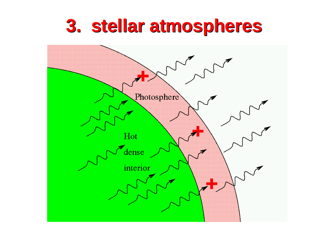 This sketch shows the basic stellar atmosphere problem. Energy is flowing in from below by convection and photons from the hot dense interior of the star. This energy flux is converted into other photons which leave the star in a transition layer known as the “photosphere”. In order to understand and predict the optical appearance of stars, we need to precisely infer the physical structure of the photosphere, i.e. its pressure and temperature structure, and we need to know the element composition.
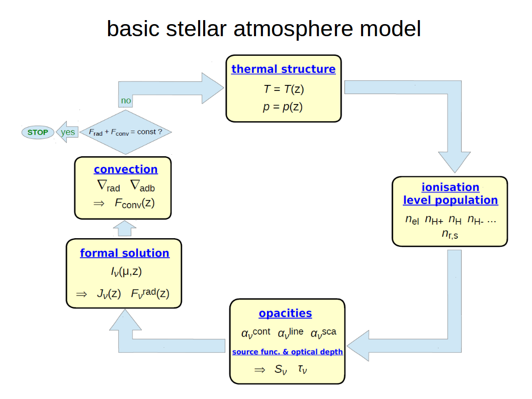 This sketch explains schematically how stellar atmosphere models work. Based on the assumed temperature/pressure structure, the abundance of all electrons, atoms, ions and molecules are computed, along with the populational numbers of their excited states. This information is then used to obtain the continuum and line opacities, including scattering. Based on the opacity structure, the equation of radiative transfer (ERT) is solved numerically to obtain a formal solution of the radiation field at all positions in the stellar atmosphere, including the observable radiative flux leaving the atmosphere at the top. We can now check energy conservation by comparing the total radiative (plus convective) flux through all layers. In radiative equilibrium, this flux must be constant in plane-parallel geometry Frad + Fconv = σTeff4 = const (“radiative equilibrium”). If it isn’t, we need to modify the assumed temperature/pressure structure in the stellar atmosphere and start all over again.
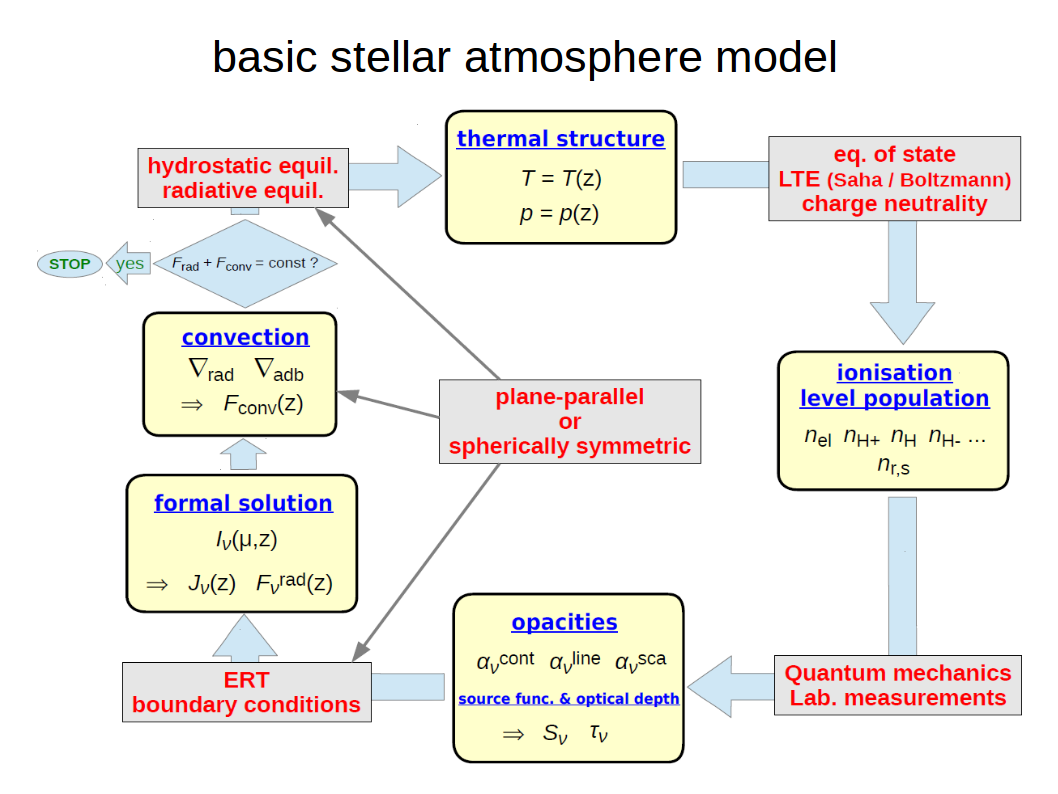 The red boxes highlight the physical assumptions and principles used in simple stellar atmosphere models.
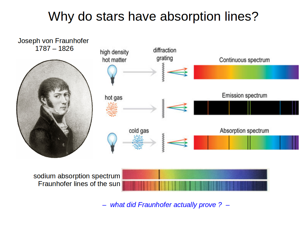 Joseph Fraunhofer (6 March 1787 – 7 June 1826) was a skillful and passionate manufacturer of optical instruments, such as lenses, prisms, and microscopes. He invented the spectrograph and discovered hundreds of dark lines in the solar spectrum, which were later identified to be atomic absorption lines by Kirchhoff and Bunsen. These lines are still called Fraunhofer lines in his honour. In the chemistry lab, it is easy to let the students see atomic emission lines by sprinkling different salts (containing different elements) over a bunsen burner and watching the emitted light through some refractory instrument like a hand spectrograph or a CD. It is less easy to demonstrate that the same lines appear in absorption if observed against a bright continuum source. The latter experiment is very close to the situation in stellar atmospheres.
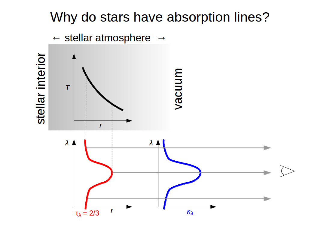 If we observe the narrow spectrum of a star around a single spectral line, the opacity in the stellar atmosphere is much larger at line centre as compared to the neighbouring continuum. Therefore, the layer which emits most of the spectral flux (τλ(r) = 2/3) is situated high in the photosphere at line centre, and deep in the continuum. One could say that the star appears to be a bit bigger at line centre. Since there is a negative temperature gradient in the photosphere, we probe cold gas at line centre, but hot gas in the continuum. Therefore, we see an absorption line. The fact that stars do exhibit absorption lines provides direct evidence for negative temperature gradients in stellar photosphere. If stars possessed the opposite, a radially increasing temperature structure, they would exhibit emission lines.
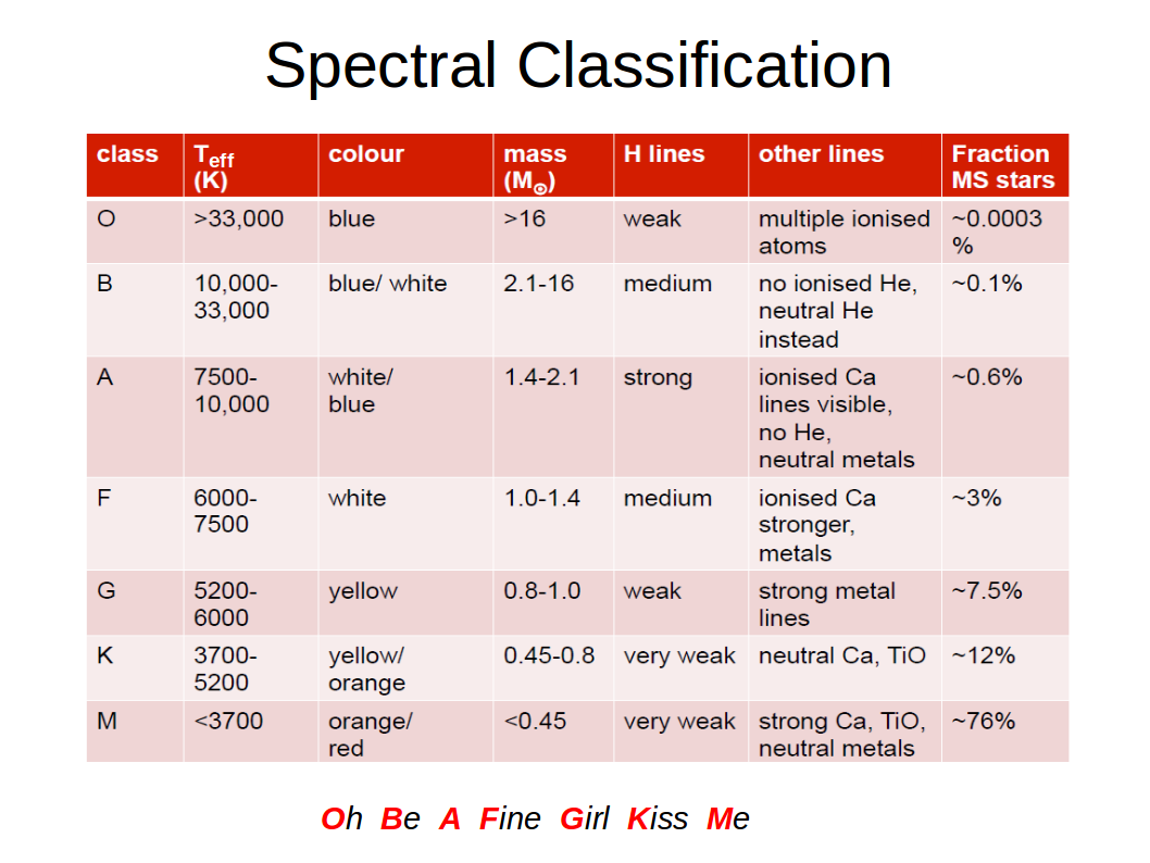 The figure summarises some stellar properties according to the Harvard spectral classification, found by observations and stellar atmosphere models. Note that the stellar mass is only valid on the main sequence (MS), whereas the associated effective temperatures and appearance of lines is also valid for giants and super-giants. There are additional letters used for carbon stars (C), white dwarfs (D), as well as brown dwarfs (L, T and Y).
Credits: St Andrews University, AS1101.
The spectra of main sequence stars
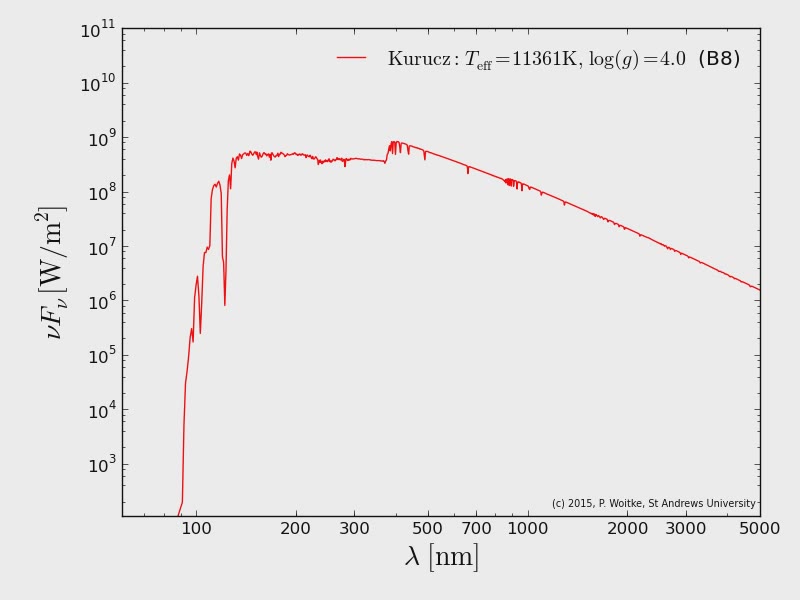
Sequence of spectra of main sequence stars from L to B-type, compiled from different tables of stellar atmosphere models (Drift/Phoenix, Phoenix, and Kurucz), which come with different spectral resolution. The x-axis is the wavelength [nm], the y-axis is the wavelength times the spectral flux λFλ = νFν [W/m2] at the stellar radius, the “surface flux”. Note the Balmer jump at 365 nm and the series of Balmer lines Hα, Hβ, Hγ, etc. occurring in particular in A-type stars.
Download the movie here
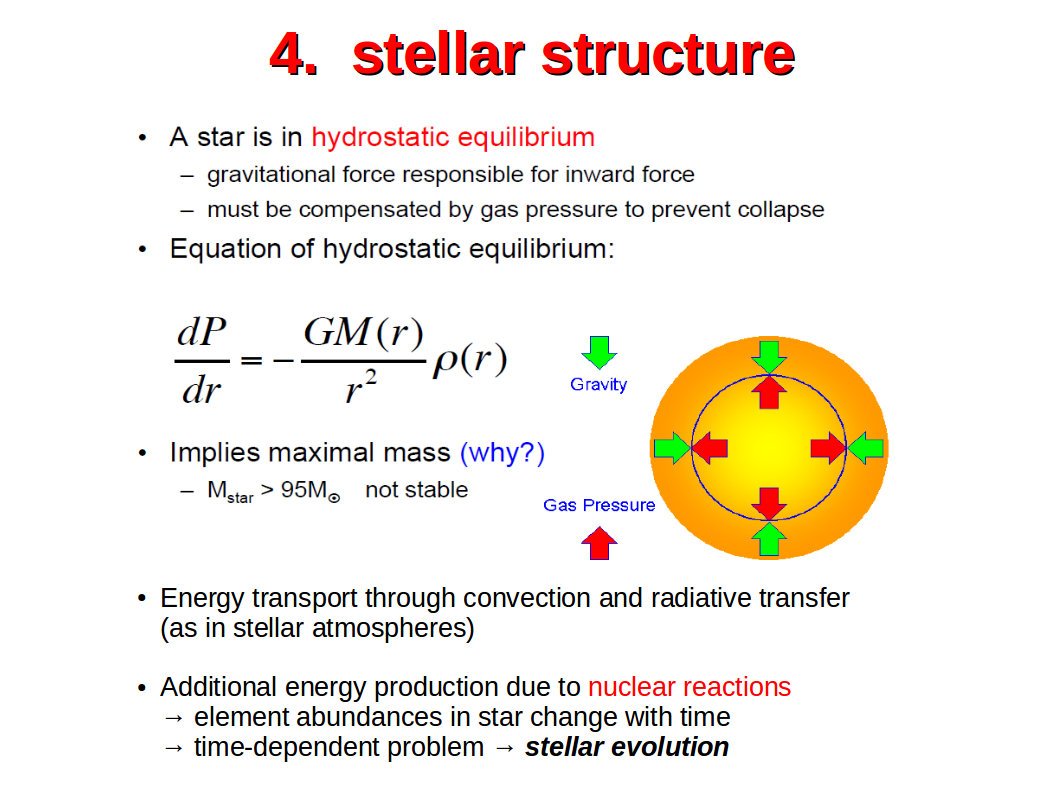 Understanding the inner structure and evolution of stars is based on similar assumptions and physical principles as explained earlier for stellar atmospheres. We assume again hydrostatic equilibrium and use similar descriptions for the radiative and convective energy transport.
However, we must consider a much more sophisticated equation of state, which remains valid even under the extreme pressure/temperature conditions in the interior of stars, and we must include one new physical phenomenon, namely the energy production via nuclear reactions. To do this, networks of nuclear reactions have been developed (the rate coefficients can be measured in particle accelerators) which predict the total local energy production rate as function of temperature, pressure, and current element abundances. Since these reactions, in return, change the element abundances, the problem becomes time-dependent.
On the main sequence, time-dependent effects are quite small, because the element abundances are still close to their primordial values. However, once hydrogen starts to get exhausted in the stellar core, things are changing. The stars will change their inner structure, change their nuclear energy production rates and start to evolve in the H-R diagram.
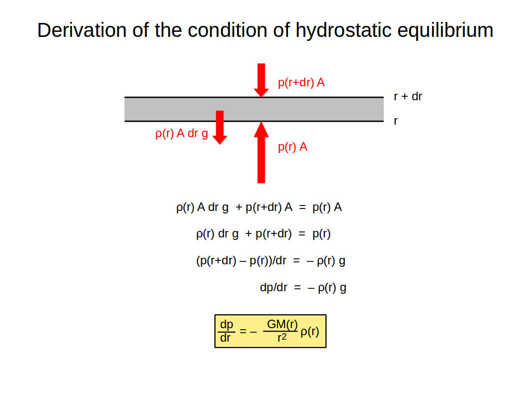 Consider a layer between r and r+dr with cross section A and mass density ρ. Write down force equilibrium (gravity, pressure from above, pressure from below), and solve for pressure gradient. Use definition of gravity g=GM(r)/r2. M(r) is the mass enclosed within radius r.
Image credits: Borb (Wikipedia)
Image credits: Borb (Wikipedia)
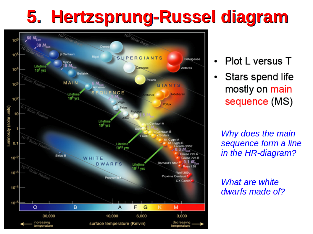 In the Hertzsprung-Russel (H-R) diagram, one plots stars with their luminosity Lstar versus effective temperature Teff (theoretical models) on double logarithmic axes, or – analogously – their absolute visual magnitude MV versus spectral class (observations). The main sequence roughly forms a diagonal line in this diagram: the overwhelming majority of all stars (called “dwarfs”) line up along this line. However, there are also “giants” and “super-giants”, which can be found in the right upper corner above the main sequence, as well as “sub-dwarfs” (denoted as white dwarfs in this plot) below the main sequence.
The H-R diagram is first and foremost a summary of observational findings, a tool by which stars can be characterised. The theoretical insight, that stars actually move along particular trajectories in the H-R diagram, is a quite recent result of research carried out during about the last 60 years, an unequalled triumph of modern science, where concerted efforts in the development of stellar computer models, particle physics (nuclear reaction rates), experimental physics (equation of state), quantum mechanics (opacities) and observations have managed to solve this puzzle in a convincing fashion, which nowadays fills standard textbooks about stars.
Note that the diagram also shows the stellar mass on the main sequence (pale magenta) and the main sequence lifetime (green). Lines with constant Rstar are also included. The sun is situated right in the centre of this plot, a G2V star with Teff ~ 5800 K and (obviously) Lstar = 1 Lsun.
Image Credits: ESO.
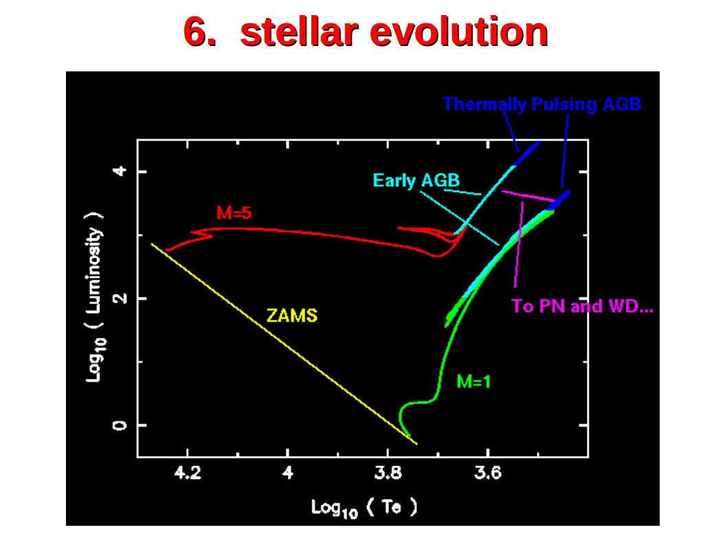 This figure shows some theoretical evolutionary tracks for low mass stars. The main sequence is marked with “Zero Age Main Sequence (ZAMS)”, because strictly speaking, main sequence stars do evolve already slightly during central hydrogen burning on the main sequence. The plot marks the very last stages of low mass star evolution in form of Early Asymptotic Giant Branch (Early AGB) stars, Thermally Pulsing AGB stars and transition to Planetary Nebula (PN) and White Dwarf (WD).
Credits: John Lattanzio (2004)
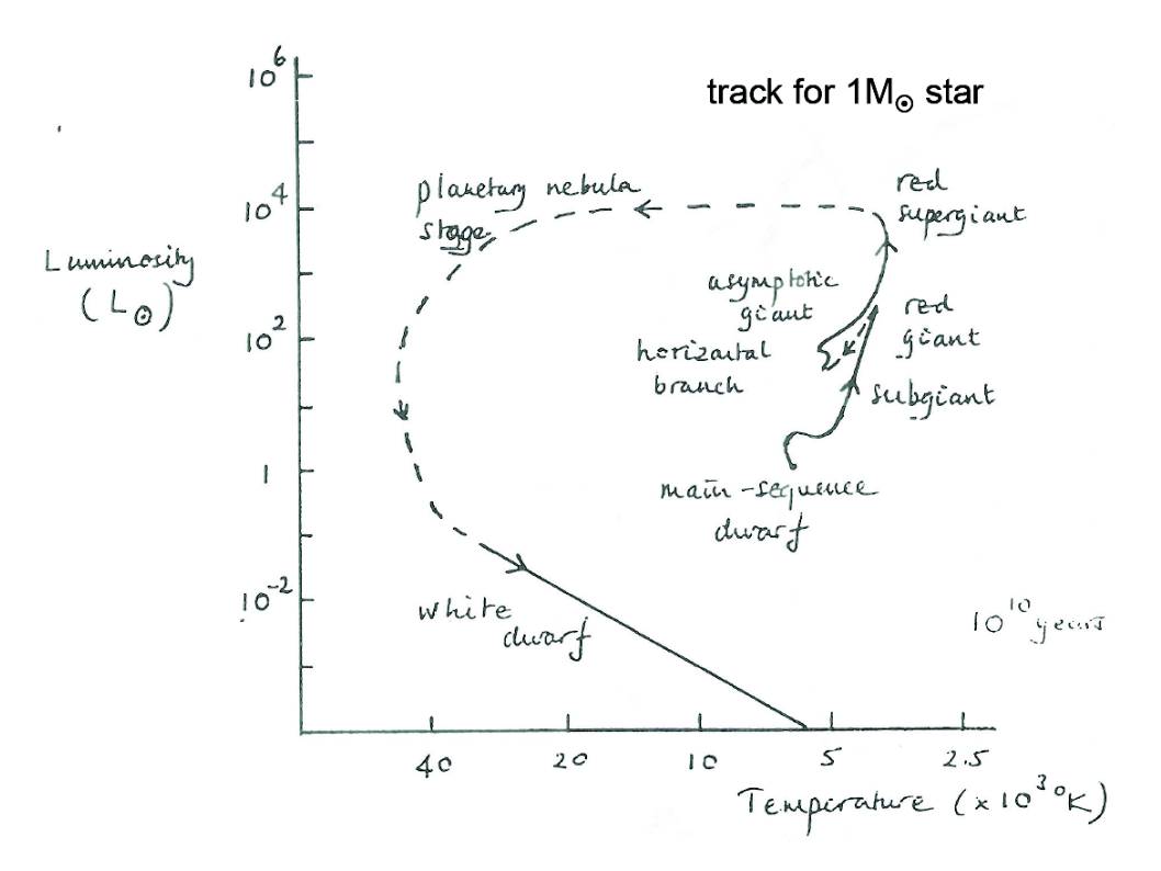 This sketch explains schematically the different phases of the life of a 1 Msun star. Once the core becomes hydrogen-poor, hydrogen starts to burn in a radial shell around the core, which causes the star to ascent along the red giant branch. At its tip, helium ignites in the core (the “helium flash”), causing the star to move temporarily leftward and downward along the horizontal branch. Finally, even helium becomes exhausted in the centre, and we find two shells with nuclear burning in the star, which causes the star to leave the horizontal branch and ascent the asymptotic giant branch. A helium burning shell above a degenerate core, and a hydrogen burning shell above those layers.
These two shells first burn in a stable fashion (Early AGB) and later in an time-dependent alternating way (thermally pulsing AGB). Low mass stars (Mstar < 8 Msun) do not reach high enough core temperatures to start burning carbon to heavier elements. However, carbon may be dredged up to the atmosphere, causing stars to become carbon-rich at the surface (carbon stars). Once the AGB stars run out of helium and hydrogen for shell burning, the stars end their lives by further core contraction (producing a white dwarf in the centre) and ejection of a planetary nebula.
Image credits: St Andrews University, AS1101.
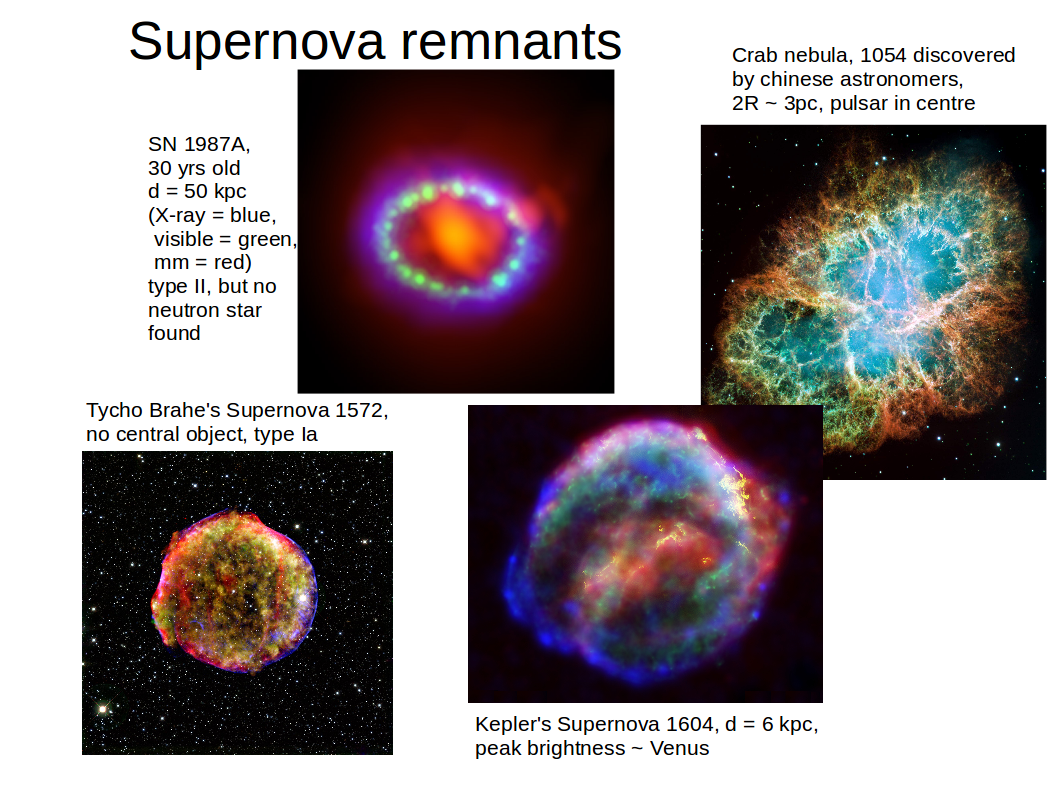
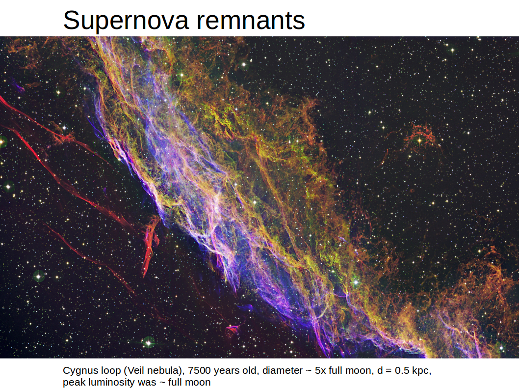
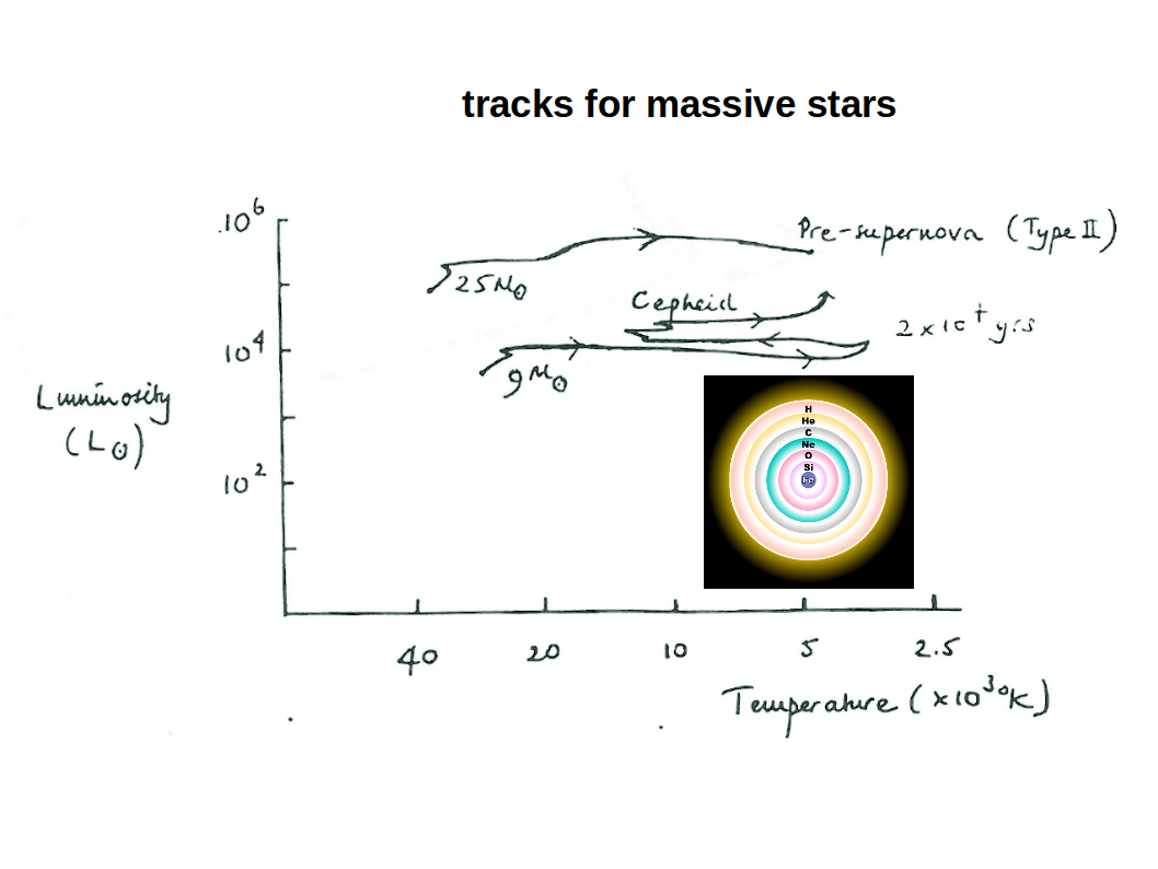 Massive stars (Mstar > 8 Msun) evolve on much shorter timescales. They start to burn He sooner, and then further to C, Ne, O, Si and eventually to Fe in distinct onion-like shells. As each major element is consumed, progressively heavier elements ignite, temporarily halting collapse. Once the nucleosynthesis process arrives at 56Fe, the continuation of this process would rather consume energy then setting free energy. Consequently, the burnt-out core can no longer withstand gravity and collapses into a neutron star in the centre, or (for more massive stars) into a black hole, whereas the envelope explodes in an spectacular supernova.
Image credits: St Andrews University, AS1101, and Wikipedia.
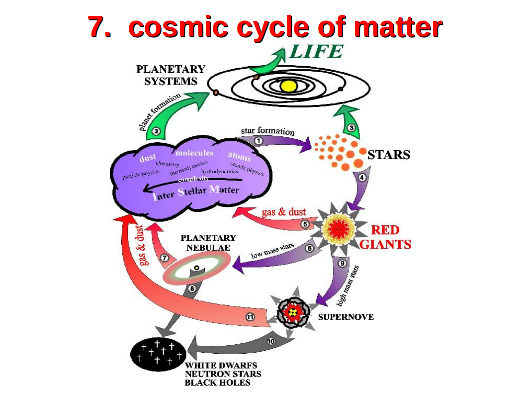 Interstellar clouds of gas and dust collapse to form stars by gravitational instabilities. Once their nuclear fuel is exhausted in the centre, they turn into red giants which blow massive winds back into the interstellar medium, partly containing processed elements and newly formed dust grains. The further evolution of the stars branches into low-mass and high-mass stars. Low-mass stars end their lives as planetary nebulae, producing white dwarfs, whereas high-mass stars explode in supernovae, partly producing neutron stars and black holes. All these phenomena, that occur when stars die, enrich the interstellar medium in heavy elements in characteristic ways.
The end products of stellar evolution (white dwarfs, neutron stars, black holes) retire from the cosmic cycle of matter, but most of the mass once confined in stars becomes available again for new star and planet formation. In fact, the sun, its planets, and all living organisms on Earth (including mankind) are made of elements that have been processed already a couple of times in the interiors of stars.
Today’s statistics show that most of the mass returned to the interstellar medium is provided by AGB star winds, but this may have been different at earlier epochs, when the universe was younger, denser, and less enriched in heavy elements. The current abundance of heavy elements such as iron, which can only be assembled in the cores of massive stars, bears witness that the matter that our world is composed off was at least once part of a supernova explosion.
Image credits: Technische Universität Berlin (2004)
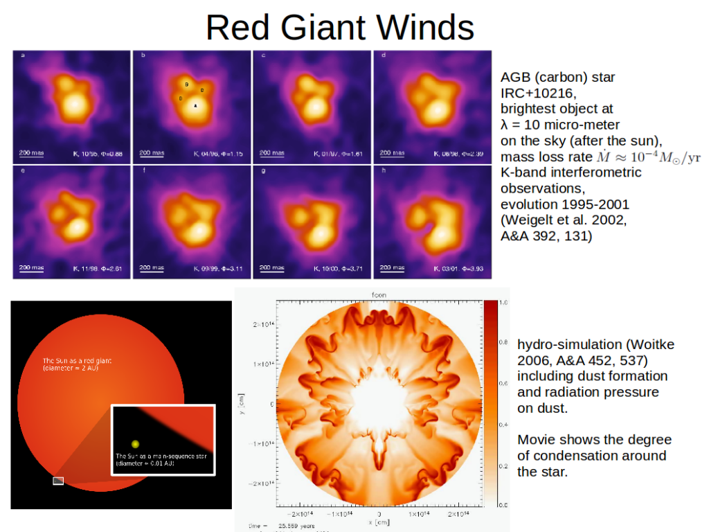
Low mass stars (< 8 Msun) loose most of their envelope mass during their final ascent along the Asymptotic Giant Branch (AGB) in the H-R diagram in form of massive stellar winds. These AGB stars are hence surrounded by large amounts of gas and dust which can become optically thick in the visual, turning these objects into pure infra-red (IR) objects, see the top figure for an example, the extreme carbon star IRC+10216, which is expected to end it’s life soon by the ejection of a Planetary Nebula. Also the sun is expected to turn into such a red giant, see lower left, with a radius of about 2 astronomical units (AU), engulfing the Earth.
The massive mass loss of these AGB stars is thought to be mainly caused by small solid particles (dust grains) forming in their outer atmospheres, which absorb the stellar photons and hence their momentum. Radiation pressure on dust can locally overcome gravity, which leads to the generation of massive slow dust-driven winds, which lifts off further stellar matter from the atmosphere.
For comparison, the sun looses about 10-14 Msun/year, i.e. 10 orders of magnitudes less than IRC+10216. Download the movie of the lower right model here. See also this page.
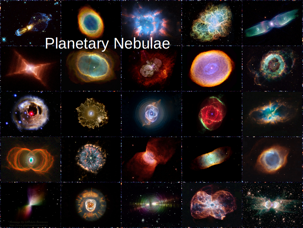 Most objects shown here are planetary nebulae, but this collection also includes other “stellar” sources such as supernovae explosions and the Wolf-Rayet star eta Carinae.
Credits: HST archive.
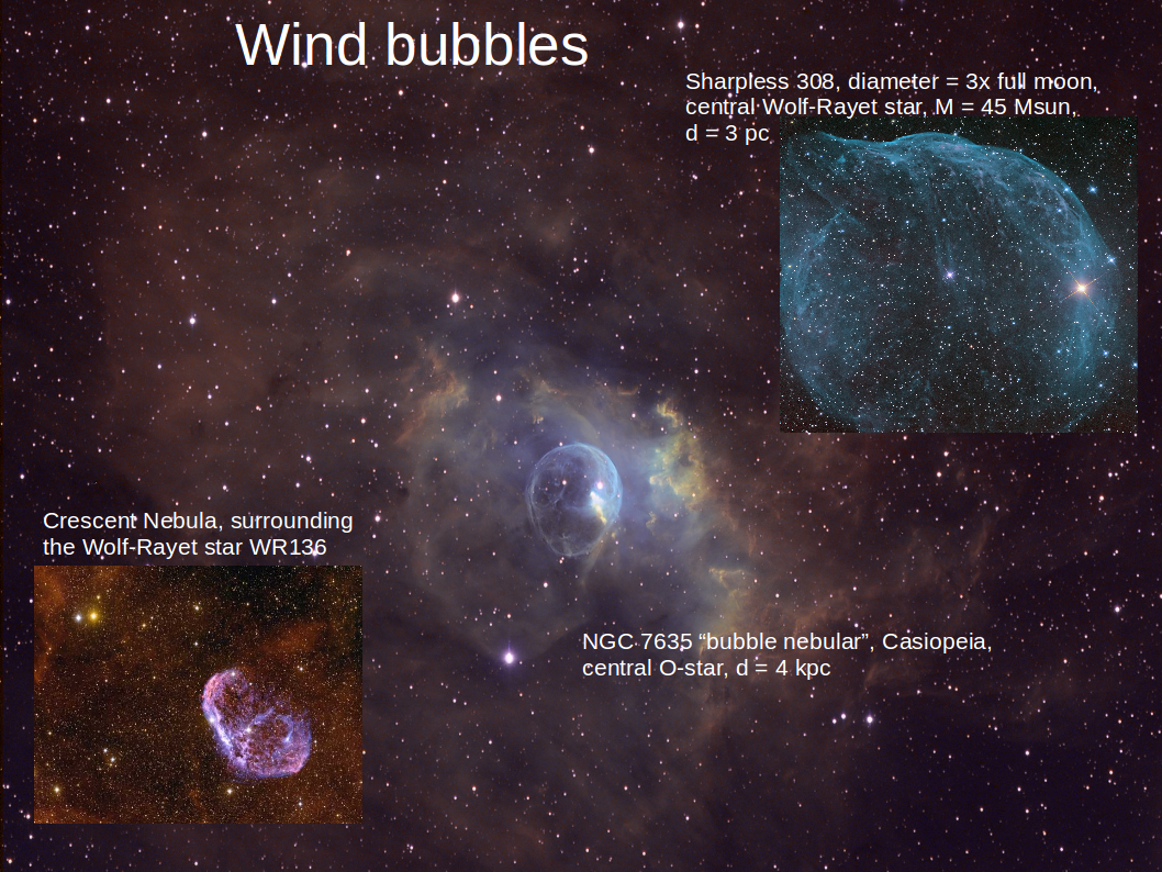 High-mass stars generate fast massive stellar winds which collide with the surrounding material from which the central stars just have formed. At the interface between stellar wind and interstellar medium, high-velocity shock waves occur which look like bubbles in emission lines.
Credits: HST archive.
 Credits: HST archive.
 Find more amazing pictures from our universe at these highly recommended websites Astronomy Picture of the Day and the Hubble Space Telescope (HST)/ESA archive. I do think that showing pictures like these to pupils of various ages may have an important, long-lasting effect on their enthusiasm for science and their aspiration for understanding our world.
Image Credits: HST archive.
Find my answers to the blue questions included in the slides here.
Peter Woitke, November 15th, 2015